FEM

Wednesday, March 31, 2021

Source of Errors in a FEM based Solution

When solving an engineering problem using FEM, we begin with developing its mathematical model. The mathematical model cannot cover all details of the physical problems, therefore, we need to simplify it and include the essential aspects of physical problem only. The mathematical model involves the solution of the governing differential equation for the system to get its exact solution which is often not possible.

The next step is to solve this mathematical model using FEM. For this purpose, we discretized the model domain into finite elements. This is equivalent to transforming the governing differential equation into a set of simultaneous algebraic equations which are solved for unknown variables to get the required numerical solution with the help of computer.

In doing above procedure, various kinds of errors are involved as shown in Figure 1.

When we represent a physical system with a mathematical model, we make several assumption. That’s why a mathematical model cannot fully describe the all details of a physical system. This is called the modelling error. The better the assumption we make in building a mathematical model of a physical system, the lower will be the modelling error.
Solution of the governing differential equation of a mathematical model is exact if we are able to solve it. Often, we resume to FEM to get a numerical solution which is an approximation. Here is the involving of discretization error. It can be reduced by increasing the mesh density at the cost of computational resources.
Lastly, whenever we compute a numerical solution, a third type of error is involved, called the numerical error. It is due to the limitation of computer memory to store numerical values. It depends on the specification of the computer system and can never be zero.

Figure 1. Sources of errors (i.e. modelling error, discretization error & numerical error) involved in getting FEM based solution of a physical problem.

Being engineer, we need to be familiar with these error sources. Let me further explain these errors with a following example.

Let’s we want to analysis the structure of an overhead storage tank as shown in Figure 2(a). The actual physical system is complex in nature and it would be rather difficult to develop a mathematical model that cover all details of this physical system. Remember we are engineers, not mathematicians, so we begin to simplify this problem to develop its mathematical model. Here are few assumptions that can make our lives at peace:

Assume that the ground behaves as a rigid body.
The inlet and outlet water piping and its connections does not contribute to the structure performance
The effect of staircase can be neglected
The weight water body can be distributed among the columns.

By applying the above assumptions, we are now able to simplify the problem as shown in Figure 2b. Whenever, we build a mathematical model of the physical problem, the modelling error is involved that depends on nature of assumptions we establish to simplify the problem. The mathematical model involves the solution of governing differential equation which do not have close-form solution in the most of practical applications. But do remember that we get an exact solution if we are able to solve the differential equation.

Figure 2. An overhead water storage tank, (a) physical problem, (b) mathematical model, and (c) discretized model.

Let’s resume to FEM to solve this mathematical model to get an approximate solution. We discretize the problem domain into finite elements as shown in Figure 2(c). During discretization, there is involvement of discretization error as we are getting an approximate numerical solution. If we discretize the model very fine, then, the discretization error will be small but the computational cost will be high. Typically, we begin with a coarse mesh, then, we keep on refining the mesh density while keeping an eye on the solution. At the onset, the solution changes drastically with increase in the mesh density until it begins to converge. At this point, a further increase in the mesh size does not affect the solution, and it is said the mesh convergence is reached. So, this discretization error is the second source of error that we should keep in mind while doing FEA of a physical problem.

The last source of error is the numerical error. This error always exist whenever we make use of computer as it has limited memory to store the numerical values being computed. This error cannot be avoided in the numerical computations due finite precision involving floating point or integer values.

In nutshell, whenever we apply FEM to solve an engineering problem, we must understand that the numerical solution we are getting is infect with various types of errors i.e. modelling error, discretization error and numerical error. Consequently, we should always doubt the solution we are getting from FEM and always try to verify or validate the results whenever possible before making a critical decision.

About the Author: Dr. Khazar Hayat is a professional engineer with almost 15+ year of experience in research, design, analysis and development of products made of fiber reinforced plastics composites (FRPCs). Currently, he is working as an Associate Professor at Mechanical Engineering Department, The University of Lahore, Pakistan, can be reaching by emailing at khazarhayat@gmail.com.

Friday, March 19, 2021

Coordinates Transformation in FEM

In this article, we will be discussing how the coordinate transformation is carried out to transform the element information i.e. element stiffness, element nodal displacements and element nodal forces, in the local/element coordinate system oriented at an angle to the global coordinate system.

This is a necessary step to be perform before starting the element assembly process. We need to check the orientation of local/element coordinate system xy-CS, used for building the element model with reference to the global coordinate system XY-CS. If the xy-CS is aligned with the XY-CS, then, we can begin the assembly of elements by constructing the element connectivity table as discussed in the previous article. Otherwise, it is essential to do coordinate transformation to align the element local information to the global coordinate system before the element assembly if the xy-CS is oriented at a certain angle to the XY-CS.

We need to transform all information of an element model i.e. nodal displacements, nodal forces and element stiffness matrix. In the below text, we discuss each of them one by one.

Transformation of Element Nodal Displacements

Let consider a linear spring element model with 2 nodes, as shown in Figure 1. Each node has 02 displacement degrees of freedom, which are represented with blue colored vectors along the element/local coordinate system xy-CS.

Please pay attention to the fact that the xy-CS is NOT aligned to the global coordinate system XY-CS, and is oriented at a certain angle. Therefore, we have to transform the blue colored nodal displacements to red colored nodal displacements which are aligned to XY-CS.

Figure 1. Transformation of element nodal displacement

Now, we discuss how to perform this transformation of the element nodal displacements. Here is the geometrical representation of the transformation between the components of nodal displacements in xy-CS and XY-CS in Figure 2.

Figure 2. Geometrical representation of the nodal displacement transformation

In terms of mathematical equations, we can write the same geometrical representation of nodal displacement transformation as following in Figure 3.

Figure 3. Mathematical representation of the nodal displacement transformation

We prefer writing all nodal displacements in the following matrix form as a matter of convenience.

Where [T] is the transformation matrix, {u'} is the nodal displacement vector in the xy-CS oriented an angle, and {u} is the nodal displacement vector in aligned with the XY-CS.

Transformation of Element Nodal Forces

In a similar fashion for the nodal displacements, we can develop transformation relation for the nodal forces as shown below in Figure 4.

Figure 4. Transformation of element nodal forces

The above information can be also present in the matrix form as below:

Where [T] is the same transformation matrix, {f'} is the nodal displacement vector in the xy-CS oriented an angle, and {f} is the nodal displacement vector in aligned with the XY-CS.

Transformation Matrix [T]

For conversion of nodal displacements and forces, we developed a transformation matrix [T] with entries of trigonometric sine and cosine ratios, shortly denoted by symbols l and m. This transformation matrix is a very special matrix because if we take its transpose or try to invert it, we get the same result. The matrix demonstrating such special property is called orthogonal matrix. Hence, the transformation matrix in our case is an orthogonal matrix as its transpose is equal to its inverse, as shown below.

The orthogonality of transformation matrix is very useful in numerical computation involving the matrix inversion. Whenever we need to inverse an orthogonal matrix, then, rather than taking its inverse we just take its transpose as inverting a matrix is a computationally expensive task as compare to taking its transpose which is merely the switching of its rows with columns. Please do remember that if a matrix is not an orthogonal matrix then we need takes its inverse as usual.

Transformation of Element Stiffness Matrix

So for we are able to develop the transformation relationships for the nodal displacement and load vectors using the transformation matrix [T], as shown below.

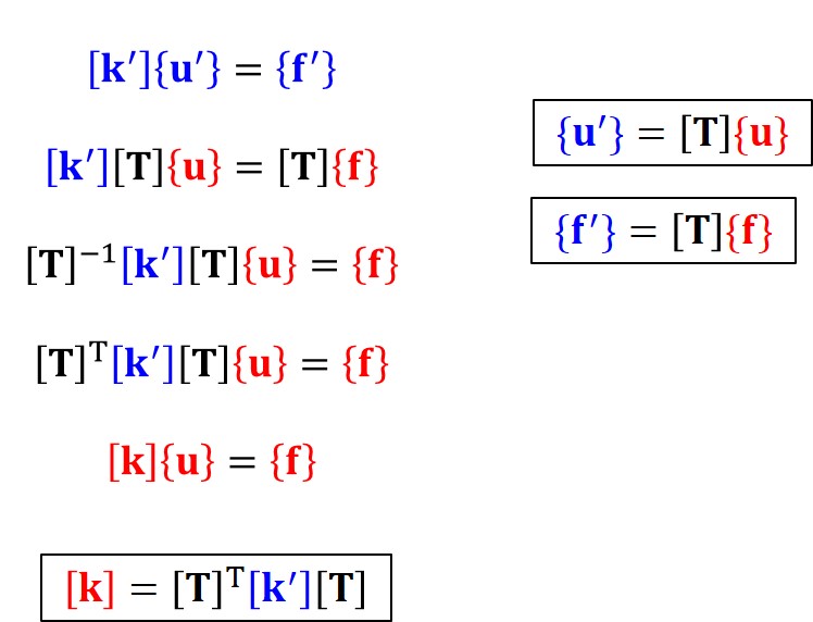
The remaining is the element stiffness matrix that also needs to be transformed from the xy-CS to the XY-CS. However, in this case use the previous transformation equations for the nodal displacements and forces, and manipulating them to derive the transformation relation for the element stiffness matrix as following.

Summary

Here is the summary of complete transformation relations for the element information in xy-CS oriented at an angle to XY-CS.

Once all element information is fully transformed from -CS to -CS, then, we proceed to the assembly process by constructing the element connectivity table. For further details on the element assembly process, please visit following article.

Monday, March 15, 2021

How a FEM software package assemble elements?

One of the strengths that makes the FEM a tool of choice is its generalized way of assembling the elements in the form global stiffness [K], and the global nodal displacement vector {U} and the global nodal load vector {F}, to build a set of simultaneous algebraic equations i.e. [K]{U} = {F}, to be solved for unknown variables.

In this article, we will go through an example problem to explain how a FEM software performs the element assembly process. The problem chosen is a linear 1D bar with legs. One of the legs is subjected to an axial tensile load while others are fixed, as shown in Figure 1.

Figure 1. A linear 1D example problem.

Let’s begin with the decomposition of the problem into small segments. Say the spatial domain of the problem is discretized into 4 subdomains so that we can easily managed their computation as shown in Figure 2. Each subdomain is assigned with an element model of a linear spring type element with two nodes, where each node has one displacement dof, as shown in Figure 3. We will not go into details of how to get this element model. Just assume that we selected it from an existing element library of the FEM software and want to use it to solve our problem.

Also, do remember that the nodes in the element model shown are local in nature. In other words, they are based on local or element coordinate system which was used to build the element model. To distinguish them from the global node numbers which we will see in the coming section, we are using a pair of braces to represent these local node numbers.

Figure 2. Discretization of the example problem.

Figure 3. A linear spring element model with local nodes to be assigned.

Now, we need to specify the global node number and element number for the discretized domain. This numbering can be arbitrary. Here is Figure 4, in which the global node number and element number used current problem are shown. The global node numbers are enclosed in circles, while, element numbers are mentioned in rectangles for distinction. Let me emphasis again, you can have your own number sequence, just do not duplicate any number.

Figure 4. Specification of global node number and element number.

After that, we have to build an element connectivity table, which simply shows the connection between the local node number, enclosed in braces, and the global node number, enclosed in circles, for each element having element number enclosed in rectangle, as shown in Table 1. This table should be read as, say for an element # 1, the local node 1 of element model is linked with the global node 4. Similarly, the second local node 2 of the element #1 is linked to the global node number 2, and so on.

Table 1. Element connectivity table.

Before starting the assembly in the form of global matrix and global vectors, we need to define the size of system. The size of system depends on the number of global nodes and number of dof per node.

Figure 5. Initialization of global stiffness matrix, and global nodal displacement and force vectors.

Finally, here begins the assembly process…

For this element we have the local stiffness matrix [k], the local nodal displacement vector {u} and the local force vector {f}, having the local size of 2x2, 2x1 and 2x1, respectively, as there are two local nodes, with each having 1 dof, as shown in Figure 6.

Figure 6. Element stiffness matrix, and element nodal displacement and load vectors.

We have to place each element of [k], {u} and {f} into their respective positions in [K], {U} and {F} initialized earlier. The positions are determined using the element connectivity Table 1, which we covered earlier. Here is the mapping of local and global positions for each entry for the element # 1.

As a consequence of above connectivity, we can see the populated global stiffness matrix [K], and global nodal displacement vector {U} and global nodal load vector {F}, with the entries of element # 1 in Figure 7 as following.

Figure 7. Global stiffness matrix, and global nodal displacement and force vectors populated with entries of element # 1.

Exactly the same process is repeated for element # 2, 3 and 4, as shown in Figure 8, 9 and 10, respectively.

Figure 8. Assembly process for element # 2.

Figure 9. Assembly process for element # 3.

Figure 10. Assembly process for element # 4.

Once assembly of all element is done, the final form of global stiffness matrix [K], global nodal displacement vector {U} and global nodal load vector {F}, can be presented in the form of [K]{U}={F}, as shown in Figure 11. This is a set of simultaneous algebraic equations, a so-called presentation of the differential equation of the system, we are looking for.

Figure 11. Final assembled form of all 4 elements.

After the element assembly, we need to apply load and boundary conditions, followed by the solving for unknown global nodal displacement. Once these unknown primary/state variables are determined, we can then compute the dependent variables as per our requirement.

Friday, March 5, 2021

Exploring FEM procedure by manually solving an Example

While performing a simulation task using any in-house developed, an open source or a commercial FEM software package, we have to follow these standard steps: (1) discretize the domain, (2) select an appropriate element type depending on the nature of the problem or develop it if not available, and assign this element model to the discretized domain, (3) assemble the elements, (4) apply the relevant load and boundary conditions, (5) solve for unknown primary or state variables, and (6) finally compute the secondary or dependent variables if required. Another terminology often used by the FEM community to describe the above steps in a more brief manner is the pre-process (i.e. step # 1 to 4), the solution (step # 5) and the post-process (step # 6).

In this article, we will be learning how a FEM simulation is conducted behind the curtain of GUI (Graphical User Interface) of a FEM software package. For this purpose, a simple structure problem shown in Figure 1 is selected. We will be solving this problem through FEM and all relevant steps involved will be performed manually to get a deeper insight of this amazing yet a powerful method. This learning journey will be a bit intensive but it will finally pay you off if you show patience.

Problem Statement

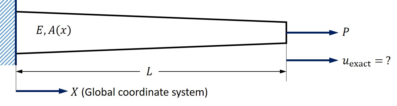
So here is the problem, we want to solve with the FEM. It is a simple bar with cross-section A(x) varying along its length L, fixed at its left end and subject to an axial load P at its right end, as shown in Figure 1. The bar is made of an isotropic material having Young’s modulus E. We want to compute the displacement u at the free end.

Figure 1. An axially loaded bar

Here is the so-called “governing differential equation” of problem along with the relevant boundary conditions.

Even though if someone is very good at solving differential equations, still, there is a slim chance to find an exact solution at the first attempt. Majority of us are not proficient at solving differential equations, that’s why, we want to solve this problem with a simple yet generalized way i.e. FEM. You will see in the following why it is so convenient to solve problem using FEM.

Finding Approximate Solution using FEM

Step # 1 Discretization

The first step in performing FE analysis involved the decomposition of the geometry of the problem (i.e. continuous domain) into simpler parts (i.e. subdomains). This process is also called meshing. Generally, all FEM software provide various mesh control options to discretize the geometry automatically or manually depending on our needs. We can also mesh the geometry outside of a FEM software or use another a software dedicated to meshing only, and import the meshed model into the FEM environment.

For the problem on hand, we will mesh the axially loaded bar into two subdomains. We can further increase the discretization, and it will surely increase the accuracy of our approximate solution, however, we limit ourselves to two subdomains only for a very good reason. And that is we will be performing the procedure of FEM manually. So here is how the discretized model looks like (see Figure 2).

Figure 2. Discretization of domain (i.e. Step # 1)

Please have a closer look at Figure 2, each subdomain has a constant cross-section. For these prismatic subdomains we already have simple solutions with which we are very much familiar in mechanics of materials course. In FEM, we are now trying to use these simple solutions for constant cross-sections, to approximate the problem with a varying cross-section along its length.

Please also note that in the above problem, we are interested in the displacement in the x-direction only, so it is 1D problem. Besides, we are using a global coordinate system for the discretized model on hand. It is named so because complete system is built using this coordinate system.

Step # 2 Develop Element Model and Assign to Discretized Domain

In this step, we have to develop an element model based on the nature of problem under investigation. In our case, the axially loaded bar behaves just like a spring. The bar deforms when loaded, and upon removal of load, it returns to its initial undeform shape.

There are numerous ways for driving an element model e.g. direct formulation, minimum total potential energy method, weighted residual method etc. Below Figure 3 shows the derivation of the element model through direct formulation method as the element stiffness matrix is derived using simple formulae of mechanics of materials. So, we model a linear spring element with two nodes. The mathematical model of a m spring element having local nodes i,j is shown below in Figure 3. The derived element model is based on a local/element coordinate system.

Figure 3. A spring element model

The next Figure 4 shows the derivation of the spring element model. Since, our focus here in not on exploring these ways of driving element model, rather than learning FEM general procedure, so we leave this discussion to another day.

Figure 4. Derivation of a spring element model.

Note that being users of a FEM software, generally we do not need to develop these element models. We have to just select an appropriate element type from the element library of the software which contains a plenty of element covering various engineering fields. The software developers have already derived and implemented these element models.

Once we developed our element model or select an element type from the element library of the software, then, we have to assign that element model to the discretized domain. Depending on the requirement of the problem, there can be more than one element type that can be assigned to various portion of the domain, but, one portion of the domain cannot be simultaneously assigned more than one element type.

In our case, we have discretized the domain into two subdomains, and each of subdomain is assigned a linear spring element with two nodes as shown in Figure 5.

Figure 5. Assignment of element type/model to the discretized domain.

Before we move ahead, it is very important to remember that the element model we developed or element type we select from the element library of the software, is built on the local/element coordinate system. For distinction, we write the local node numbers of element in the braces. On the contrary, the discretized model is built on the basis of global coordinate system, and therefore, we write the global node numbers of the discretized model in circle to make a clear distinction.

We do we need to make above distinction? Because the element model is built in local/element coordinate system. When we assigned the elements to the discretized model built in global coordinate system, we have to transform the relevant attributes of the element from local to global coordinate system.

Step # 3 Assembly of elements

The next step involved in a general procedure of FEM, is to assemble the elements which were previously assigned to the discretized domain. In doing so, we need to map the local node numbers of the elements to the global node numbers in the system. This is done in the form of an element connective table as shown n Figure 6. The first column of the table lists the element number of elements in the discretized domain. The next columns list the global node numbers and corresponding local node numbers for each element.

Table 1. Element connectivity table

Before, we start to assemble the elements, an empty global stiffness matrix, a global displacement vector and a global load vector, each populated with zero values, is constructed. The size of the global matrix and the global vectors is based on the number of global nodes (i.e. 3 in our case) and number of degrees of freedom per node (i.e. 1 in our case), and is determined as shown in Figure 6.

Figure 6. Sizing of global stiffness matrix and global vectors.

With the help element connectivity table, we transform the local stiffness matrix of each element to corresponding global stiffness matrix. After the completion of this operation, we add the elements of global stiffness matrix of each element to get the global stiffness matrix of the system, as shown in Figure 7. Likewise, we construct the global nodal displacement vector and the global nodal force vector.

Figure 7. Assembly of elements

Here is the final form as shown in Figure 8, the assembled elements in the form of a set of simultaneous algebraic equations, and computers are very very good at solving such system of equations without getting bored.

Figure 8. System global stiffness matrix, nodal displacement vector and nodal force vectors.

Step # 4 & 5 Apply load & boundary conditions and Solve for unknown Primary variables

Before we proceed further we need to apply the load and boundary conditions. There is a tip load at global node number 3. The displacement of global nodal number 1 is zero as this node is fixed boundary condition. There is no external force on global node number 2, so it will have net zero nodal force, as shown in the upper portion of Figure 9.

After the application of load and boundary conditions, the set of simultaneous equations is solved for unknown primary variables i.e. displacement dof at each node. The computer solve the set of simultaneous equation of the form Ax = b, by inverting the matrix A and multiplying it to vector b. To inverse a matrix, it should be not a singular matrix because a singular matrix cannot be inverted.

Figure 9. Application of load and boundary conditions, and solve for unknown primary variables.

Step # 6 Compute Dependent or Secondary Variables

The last step is an optional post-processing step. It includes result visualization, data plotting, or computation of the secondary variables from the primary variables etc. The example of computed secondary variables in the current problem could be the strains which can then be converted into stresses using the constitutive relationship at the element level, as shown in Figure 10.

Figure 10. Compute dependent or secondary variables.

Sunday, February 28, 2021

How to select an Element Type in performing FE analysis?

An element is fundamental building block of a finite element model and its proper selection plays a pivotal role in analyzing the problem on hand. In this article, I would explain the types of elements and their properties that will help you to make a better selection for your FE analysis.

Properties of Elements

An element represent a subdomain of engineering problem. The vertices of elements are called nodes. Sometimes, extra nodes are also located inside elements. These nodes serves following purpose:

Element Geometry

The geometry of elements can be defined by proper placement of its nodes. They can have 1D, 2D or 3D dimensions. The number of nodes increases with increase in the element dimensionality thus require more computational resource.

In structural applications, the 1D structure elements are better suited for FE modeling of long prismatic sections like rod, pipe, beam etc. where length dimension is significantly larger than the cross-section dimensions. For plan stress or strain problems of shell and plates etc., where length and width dimensions are much larger than thickness, 2D structural elements can better for FE idealization. The 3D structural elements are generally use to analysis the structures where all three dimensions of are comparable or there is need to investigate in detail complex 3D state of stress or strain.

Figure 1. Geometry of 1D, 2D and 3D structural elements

It is interesting to note that there are some special elements which have no dimensionality like lumped spring, point mass, contact elements etc. Such elements are used in an abstract way during FE modelling, so be ready face this reality.

Element Response

The response of elements is governed the attributes of its nodes. The nodal attributes are the unknown primary or state variables in the FE model that are computed at nodes, that’s why, these are called nodal displacements or nodal degrees of freedom (dofs), and are represented with {u}. There is one-to-one correspondence between the nodal dofs {u} and associated nodal forces {f}, and this defines the constitutive relationship at the element level i.e. {f} = [K]{u}, and the element response is dictated by this constitutive model working behind it.

In nutshell, the element response is expressed in terms of its dofs which are calculated during analysis. For structural elements, the dofs are displacement and rotations at each node, for thermal elements, the dof is temperature.

Selecting of a Right Type

When you want to build a FE model, you should use your engineering knowledge and judgement to identify the key variables that govern its behaviors. Say, you want to do a coupled thermal-stress analysis of a product. The geometry of product is such that all its dimensions are comparable. For this case, a 3D element would better idealize its geometry. Next, requirement would be to make sure that the selected 3D elements have relevant dofs that can capture the required coupled thermal-stress interaction i.e. temperature dof in addition to displacement degree of freedom to capture the coupled thermal-stress interaction.

Never trust your memory, always consult manuals of a commercial software packages to find appropriate element types for your FE model. The manuals not only list in detail the attributes of elements, its applications and limitations, and its formulation but also provides guidelines and example problems.

How to perform Finite Element Analysis (FEA)?

Whether you are an expert or novice, irrespective of the type of problem belonging to any engineering discipline you want to solve, regardless of using your own FEM tool or an open-source software or a commercial package, you have to follow the these standardized steps to complete your FE analysis.

In this article, I would explain the essential steps involved in completing your FEM based analysis.

Essential steps to conduct Finite element analysis (FEA)

The first step involved the decomposition of the problem domain into small finite subdomains, called elements. The power of FEM lies in its ability to discretize a complex continuous domain into finite elements and nodes. This process is also called meshing. The purpose of meshing process is to prepare a set of unknown variables to be determined over the entire domain where solution is to be obtained.
Select an appropriate mathematical model i.e. governing differential equation, related to your analysis type and convert it into element model by using FEM. Assign these elements to the discretized domain. Say, you are solving structural problem, then, you have to develop your own structural element or choose from already available catalogue of elements, and assign it to the discretized domain along with relevant material properties.
During this step, the stiffness matrix of each element is assemble into a global stiffness matrix representing the entire discretize domain.
Apply loads and boundary conditions.
Solve for unknown displacement vector (i.e. primary or state variables).
Calculate dependent or secondary variables, if required.

Figure 1. A general procedure for Finite Element Method (FEM) based analysis.

The procedure of performing FEA using above steps seems very cumbersome, but, in actuality it is not. Many commercial software packages have been develop to simplify the FEA. For commercial tools, the above steps, also shown in Figure 1, can be categories as following stages:

Preprocess
This stage covers step# 1 to 4 listed above. The geometry of problem is either modelled in FEA software, or may be imported. Then, it is meshed. There are meshing tools available in the software packages which mesh automatically but also manual mesh control. After meshing, the element type is selected for already developed catalogue of elements depending on the nature of analysis to be perform. These elements are assigned to the meshed domain along with relevant material properties. Next, appropriate load and boundary conditions are defined.

Solution

At solution stage, an appropriate solver is selected to find out the unknown displacement variables. A solver is an algorithm that efficiently solves a big set of simultaneous algebraic equations to compute unknown state variables.
Post-process
It involved the derivation of dependent or secondary variables from primary or independent variables, and plotting and visualization of results as per requirement.

How Finite Element Method (FEM) Works?

Background

Over the period of time the Finite Element Method (FEM), also known as Finite Element Analysis (FEA) has become a default tool in the Computer-Aided Engineering (CAE) design process of products and systems. Engineers, all over the world, are deploying this powerful tool to analysis real life engineering problems. The applications of FEM are huge and diverse ranging from structural, thermal and fluid flow problems, to electrostatics and magnetostatics and so and so on.

The significance this essential tool in today’s modern world cannot be emphasize more. However, it is ironic that the engineering students (the potential future users of this tool), are often taught to perform design and synthesis for simple problems with ideal applications only. They are taught to learn engineering principles, build mathematical models and solve these simple problems. On the contrary, after graduation they are expected to solve the real world problem which are complex in nature and often expressed by scary-looking mathematical equations (so-called governing differential equations) which may not be solved easily or its exact solution (close-form solution) may does not exist. Here comes a much need FEM tool in the arsenal of fresh engineers to rescue them…

In this article, I would explain how this amazing tool works to solve complicate engineering problems using a typical structural problem. The target audience of this article are undergrad students and/or and new engineers who have a little or experience with FEM. The article may also serve as a reminder of the basic concept behind the FEM for the experience users.

FEM is based on "Divide and Conquer" Philosophy

The underlying idea of FEM is similar to “divide and conquer”. We treat a complex problem as a set of simple problems which can be solved easily. Let me explain it further with an example shown below in Figure 1. A prismatic cantilever beam is subjected to a tip load P at its free end, and we want to compute its deflection. The term prismatic is a fancy terms dedicated for the structural components which have constant cross-section along its length. The general differential equation of beam that governs it is as following:

Even though above equations seems complicate, but, it can be solve it for the given square cross-sectional prismatic beam by applying the following boundary conditions.

We were lucky to have solution for the above case. Such way of approaching the problem by solving differential equations derived for a continuous domain is called analytical modeling. In reality, the cross-section of beam may be not rectangle type or not even prismatic or may be it is made of composite materials etc. There are unlimited possibilities for even a single structural beam which could not be coped with analytical models. That is why the exact solution of the real world engineering problem generally do not exist. This is alarming for us being engineers.

Figure 1. The defection of prismatic cantilever beam using analytical method (Differential Equation) and numerical method (i.e. FEM)

In case of FEM, we decompose the continuous domain of the problem, which is the cantilever beam in our case, into simple subdomains, called finite elements or shortly elements, hence is the name of this approach the Finite Element Methods (FEM). Every finite element has nodes through which it connects with other elements. In above example, each element consists of two nodes. Every finite element represent an algebraic equation for a subdomain in the finite or discretized domain. In other words, the whole finite domain is now expressed mathematically in terms a set of simultaneous algebraic equations, generally, denoted in vector and matrix notation as following:

Where vector {F} is called force vector, {U} is load vector and [K] is called stiffness matrix. The size vectors and matrix (i.e. a set of simultaneous equations) depends on the number of elements in the domain.

The stiffness matrix represent the system properties of the domain, and displacement vector represents the behavior of the domain subjected to force vector. The displacement vector is also called nodal displacement vector, state vector or degree-of-freedom (dof) vector. The solution of unknown displacement vector is obtained by solving for given the known load vector and stiffness matrix as following.

It might be also interesting to you that the above notation used for representing a set of simultaneous algebraic equation is only well understood in mechanical and civil engineering disciplines, but also very popular in other disciplines where it represents other quantities as depicted in this following Table 1.

Table 1. Use of FEM in other disciplines.

Application Problem	Displacement vector represents	Force vector represents
Solid mechanics	Displacement	Mechanical force
Heat conduction	Temperature	Heat flux
Acoustics	Displacement potential	Particle velocity
Flow problems	Pressure	Particle velocity
Electrostatics	Electric potential	Charge density
Magnetostatics	Magnetic potential	Magnetic intensity

Coming back to our discussion on the solution of simultaneous algebraic equations, let me highlight that we have already learnt how to solve these equations manually in our elementary mathematics class during school education. We were able to solve a set of 2 or 3 simultaneous algebraic equations only, however, the solution of a big set is humanly impossible, at least to me.

Fortunately, the computers are very good at doing boring jobs. Computer do arithmetic operations that are only needed to solve simultaneous equations involving the inversion of stiffness matrix. Numerical algorithm are available to inverse a stiffness matrix considering time and memory constraints. Modern computers have the capability of solving rapidly huge set of simultaneous equations as all it require is the computational power and efficient algorithms. Consequently, with the development of computer, we are feel empower to analysis the huge and complicated engineering systems and their interactions with the power of FEM.

Being users of FEM, it is very important for use to understand that such numerical solution is an approximate solution. The accuracy of FEM solution depends on the number and the type of elements. Here I will explain the role of the number of elements only as the type of elements is beyond the scope of this article. The number of elements in domain increases as we enhance the discretization of domain from course to fine. The accuracy of solution generally increase with increase in the number of elements, however, a stage will come that an increase in the number of elements will no longer increases the accuracy of the solution, such condition is said to be mesh convergence. A further increase in number of elements will increase the size of the set of simultaneous equations, which will become a computational intensive and time consuming task, but, with no proportionate improvement in the solution. We, being users, should have to strive for a reasonable approximate solution at optimal utilization of resources.

FEM